The dollar sign ($) in Excel tells Excel to change or not to change a cell reference when a formula is copied to another cell. This tutorial will guide all levels of Excel users on how to manipulate absolute and relative references in Excel and Mac.

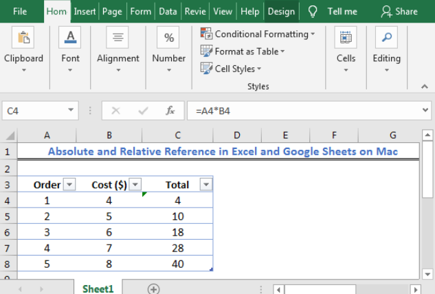
Figure 1: Absolute and Relative Reference in Excel and Google Sheets on Mac
*** To copy down a formula, click on the cell with the formula, at the bottom right, you will see a small box. Take your cursor to the box. Now you will see a + sign. Left-click your mouse and drag down the + sign.
A relative cell reference is Excel is a Cell address without the dollar sign in the row and column as we copy down the formula. As we copy down a formula with a relative cell reference, the cell reference changes based on the rows and columns relative positions.

Figure 2: Relative Cell reference in Excel
As shown in figure 2, the returned result in Cell C4 is for the multiplied values referenced in Cell A4 and Cell B4 . The formula looks like this:
Cell D4: =A4*B4
Cell D5: =A5*B5
Cell D6: =A6*B6
Cell D7: =A7*B7
Cell D8: =A8*B8
What is an Absolute Reference?
An absolute cell reference is Excel is a Cell address with the dollar sign in the row and column as we copy down the formula. As we copy down a formula with an absolute cell reference, the cell reference remains unchanged regardless of the row and/or column.
How to Do Absolute Reference in Excel

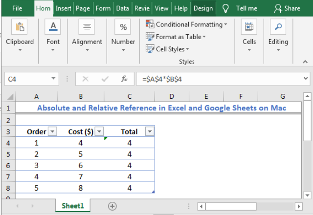
Figure 3: Absolute Cell reference in Excel
As shown in figure 3, the returned result in Cell C4 is for the absolute multiplied values referenced in Cell A4 and Cell B4 . The formula looks like this when copied down:
Cell D4: =$A$4*$B$4
Cell D5: =$A$4*$B$4
Cell D6: =$A$4*$B$4
Cell D7: =$A$4*$B$4
Cell D8: =$A$4*$B$4
A mixed cell reference in Excel is a Cell address that has either the column letter or row number fixed. This means that either the column letter or row number is locked or absolute referenced , e.g. in $A1, Column A is locked but row 1 is relative.

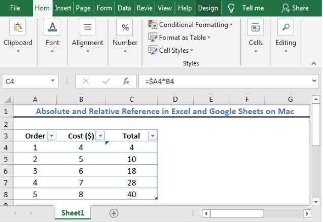
Figure 4a: Mixed Cell reference in Excel
As shown in figure 4a, the returned result in Cell C4 is for the multiplied values with a mixed column (Column A) reference in Cell A4 and Cell B4 . The formula looks like this when copied down:
Cell D4: =$A4*B4
Cell D5: =$A5*B5
Cell D6: =$A6*B6
Cell D7: =$A7*B7
Cell D8: =$A8*B8
If we add the dollar sign to the row number of Column A, the result will look like this:

Figure 4b: Mixed Cell reference in Excel
As shown in figure 4b, the returned result in Cell C4 is for the multiplied values with a locked reference for Column A and Row 4 in Cell A4 and Cell B4 . The formula looks like this when copied down:
Cell D4: =$A$4*B4
Cell D5: =$A$4*B5
Cell D6: =$A$4*B6
Cell D7: =$A$4*B7
Cell D8: =$A$4*B8
In the example below, we will see that although Column B is a relative reference, because Row 4 is locked in the formula, our result is always returned as 4 .

Figure 4c: Mixed Cell reference in Excel
The formula in figure 4c remains $A$4*B$4 when copied down.
Note: Pressing the F4 key without selecting any cell reference causes the reference to the left of the mouse pointer to be automatically selected. This results in a change to another reference type.
For Mac, we can use the shortcuts below:
fn + F4
Most of the time, the problem you will need to solve will be more complex than a simple application of a formula or function. If you want to save hours of research and frustration, try our live Excelchat service! Our Excel Experts are available 24/7 to answer any Excel question you may have. We guarantee a connection within 30 seconds and a customized solution within 20 minutes.